5 Stochasticity
This chapter will give an introduction to stochastic environments and bet-hedging strategies. The underlying theory is based on stochastic processes and probability theory, and this chapter will only touch upon a few basic concepts from this large research field. A key result from the most basic model of stochastic population growth is that the long-term population growth rate (fitness) in variable environments will always be lower than the growth rate in the constant mean environment.
5.1 Learning goals
Understand key properties of population growth in variable environments.
Describe the main properties of the Lewontin-Cohen model.
Understand how bet-hedging strategies can help individuals live in variable environments.
Discuss the role of variable and unpredictable environments in light of climate change.
5.2 Variable vs unpredictable environments
So far we have only considered populations in constant environments. But natural environments can be highly variable, both in time and space. Here, ‘environment’ is a very general term which can refer to any particular abiotic variable (like temperature) or a combination of several factors that affect organisms living in the habitat, including biotic factors like resource availability. Environmental variability can be predictable, like the seasonal changes in light conditions at high latitudes, or unpredictable - which is the case for stochastic environments. Unpredictable variation also includes rare events such as rainfalls in a dessert, or flooding and wildfires. We can estimate a frequency at which such events typically occur over many years, but it is difficult to predict the exact timing of each such event.
Practically all organisms live in some kind of variable environment (although some habitats are more stable than others, for instance the deep depths of the oceans), and species have evolved various strategies to deal with both the wide range of possible conditions they (or their offspring) may encounter, under varying degrees of predictability. These adaptations allow individuals to mitigate negative impacts of bad conditions, as well as take advantage of good conditions, and spread the risk associated with uncertainty in various ways.
If the environment is fluctuating in a predictable way, phenotypic plasticity can allow individuals to cope with the variation. Organisms can then take advantage of environmental cues during development to achieve an optimum phenotype in the future environment. For unpredictable (stochastic) environments, however, organisms cannot rely on such cues. In these cases bet-hedging strategies may evolve.
5.3 The Lewontin-Cohen model
The simplest model for stochastic population growth applies to an unstructured population. In this model the annual population growth rate is a stochastic variable \(\Lambda_t\) with mean \(\text{E}[\Lambda_t]=\lambda\), variance \(\text{Var}(\Lambda)=\sigma^2\), and with no autocorrelation between the growth rates of different years. This means that the annual growth rates are IID (Identically and Independently Distributed), and this assumption is important for the derivation of the long-term population growth rate. This model is the Lewontin-Cohen model (Lewontin and Cohen 1969), also known as a ‘geometric random walk’.
5.3.1 Defining the process
Starting from a population size \(N_0\), the population size after \(t\) time steps in the Lewontin-Cohen model is given by
\[\begin{align} N_{t+1}=\Lambda_{t}\Lambda_{t-1}\cdots\Lambda_{1}\Lambda_0N_0=N_0\prod_{i=0}^t \Lambda_i. \tag{5.1} \end{align}\] We are interested in the behavior of a ‘typical’ population growing according to this process, and to define the long-term growth rate of such a ‘typical’ population (the socalled stochastic growth rate). As we will see below, this is not the growth rate of the mean population size, but rather the median population size. Before we go into details of this derivation, we will look at how we can generate realizations of the Lewontin-Cohen process in R and plot one or more realizations.
Plot one realization of the process
The R function LC below can be used to generate a random sequence of population sizes over time based on this model (each time you run the code it will generate a different sequence, unless you use the function set.seed() which initializes the pseudorandom number generator in R). The LC function returns the sequence of population sizes as a data frame, including the time steps from 0 to the set number of years. The output from one run of the function is shown in figure 5.1. In this example, a normal distribution is used to generate the sequence of annual growth rates, but the exact kind of distribution is not critical as long as the mean and variance can be set independently (for instance, a lognormal distribution could be used since all the multiplicative growth rates should be non-negative).
#mean.lambda: Expectation of annual lambda
#sd.lambda: Standard deviation of lambda

LC <- function(Tmax=30,
               n0=100,
               mean.lambda=1.05,
               sd.lambda=0.1){
  stochastic.lambdas <- rnorm(Tmax,
                              mean=mean.lambda,
                              sd=sd.lambda)
  Nvec <- rep(NA, Tmax+1)
  Nvec[1] <- n0
  for(i in 1:Tmax){
    Nvec[i+1] <- stochastic.lambdas[i]*Nvec[i]
  }
  data.frame("Time"=0:Tmax, "N"=Nvec)
}

#Initialize R's random number generator,
#the number chosen is arbitrary
set.seed(20)

#Apply function and plot result:
StochasticGrowth <- LC()

ggplot(StochasticGrowth) +
  geom_line(aes(x=Time, y=N), lwd=1.2)+
  geom_point(aes(x=Time, y=N), size=3)+
  theme_bw() +
labs( x="Time (year)", y="Population size N") 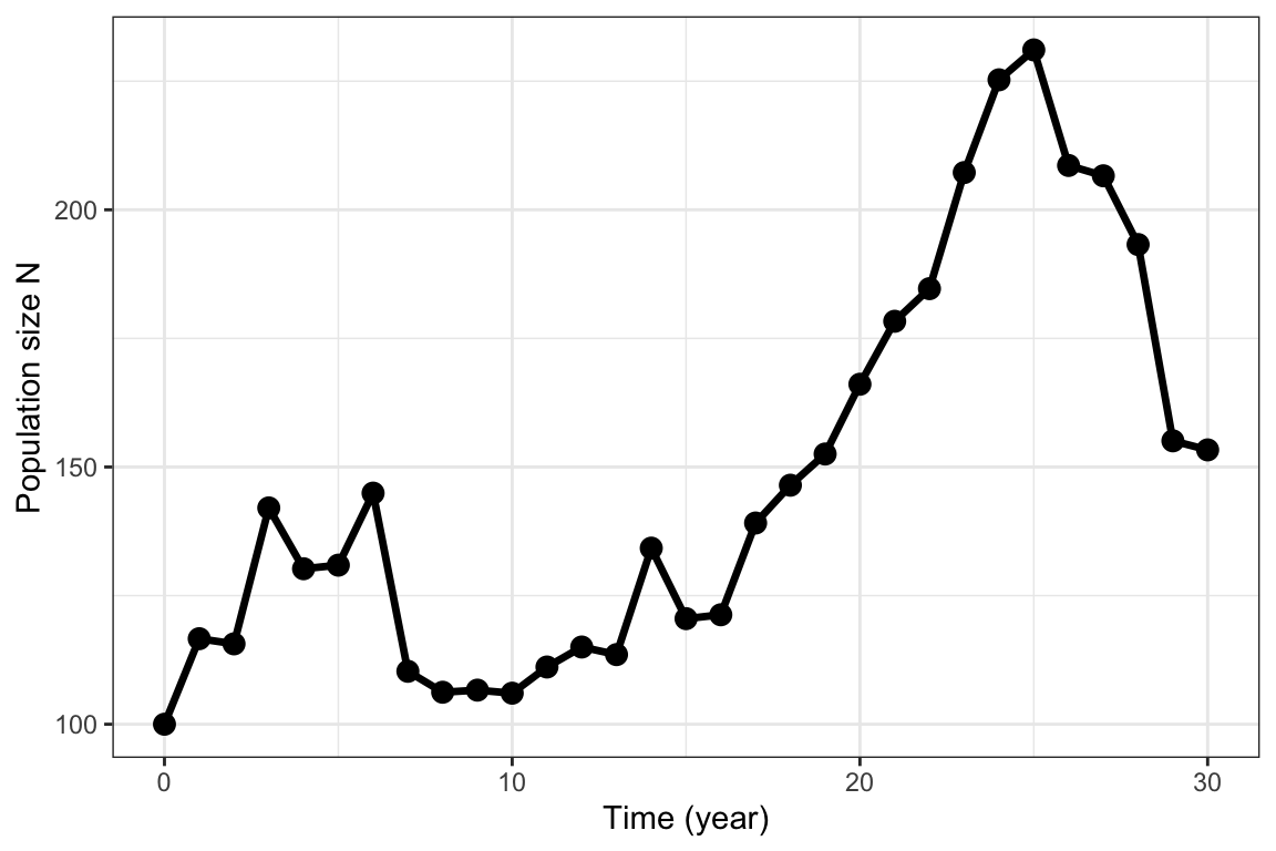
Figure 5.1: Stochastic population growth following the Lewontin-Cohen model with normally distributed annual growth rates with mean \(\lambda=1.05\) and standard deviation \(\sigma=.1\)
This code only generates one realization of the growth process. To learn more about the typical behavior of this stochastic growth process we need to generate many realizations (from the same starting point, with the same mean and variance of the annual growth rate) and look at some summary statistics.
Plot many realizations of the process
The following function generates a chosen number (nsim) of realizations of the Lewontin-Cohen model, stores them in a data frame and makes a plot of all of them.
nsimLC <- function(nsim=100, Tmax=30, n0=100,
                   mean.lambda=1.05, sd.lambda=0.1){
  frame <-  data.frame("Time"=0:Tmax)
  for(j in 1:nsim){
  stochastic.lambdas <- rnorm(Tmax, mean=mean.lambda, sd=sd.lambda)
  Nvec <- rep(NA, Tmax+1)
  Nvec[1] <- n0
  for(i in 1:Tmax){
    Nvec[i+1] <- stochastic.lambdas[i]*Nvec[i]
  }
  frame <- cbind(frame, Nvec)
  names(frame)[j+1] <- paste("N",j,sep="")
  }
  frame
}
To apply this function and plot the results, we can use the following code:
set.seed(20)

simLC100 <- nsimLC()

simLC100.long <- simLC100 %>% pivot_longer(c(-Time),
               names_to = "Rep", values_to = "N")

ggplot(simLC100.long) +
  geom_line(aes(x=Time, y=N, col=Rep), lwd=.5)+
  scale_color_manual(values=rep(1,100))+
  theme_bw() +
   theme(legend.position = "none" )+
labs( x="Time (year)", y="Population size N") 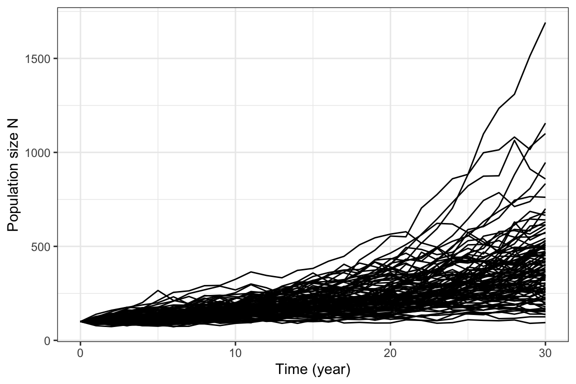
Figure 5.2: 100 realizations of the Lewontin-Cohen model with normally distributed annual growth rates, with mean \(\lambda=1.05\) and standard deviation \(\sigma=.1\)
Figure 5.2 shows the output from 100 realizations. We see that over time, these realizations diverge more and more from each other as the randomness accumulates. A few realizations reach large population sizes, while many are located in intermediate values. However, it quickly gets quite messy to plot so many realizations, and if we want more than 100 it will be even worse. If we want to summarize the outcome of many realizations over time, a better option is to plot selected percentiles over time.
Plot percentiles from many realizations
Percentiles (or quantiles) are useful for summarizing outputs from many realizations. For instance, the 50%%% percentile represents the population size at which 50\(\%\) of the realizations will lie above it and 50\(\%\) below it (i.e. the median in the limit as the number of realizations approaches infinty), the 95\(\%\) percentile represents the population size at which 5\(\%\) of the realizations lies above it and 5\(\%\) below it, etc. The following code makes such a plot based on 10 000 realizations of the Lewontin-Cohen process. It can take some seconds to run (reduce the number of realizations nsim if it gets too slow)
#Apply function to get 10 0000 realizations (can take some time)
simLC_Large <- nsimLC(nsim=10000)

#Get the 5, 25, 50, 75, and 95 percentiles:
Percentiles1  <- t(apply(t(simLC_Large[,-1]),
                         2,
                         quantile,
                         probs=c(.05, .25, .5, .75,.95)))


#Store percentiles in data frame
LCPercentiles <- as.data.frame(cbind("Time"=0:(dim(Percentiles1)[1]-1),
                                     Percentiles1))

LCPercentiles$Mean <- apply(t(simLC_Large[,-1]),2, mean)

#Make long format for plotting
LCPercentiles.long <- LCPercentiles %>% pivot_longer(c(-Time),
               names_to = "Percentile", values_to = "N")

#Make sure the order of the percentiles is correct
LCPercentiles.long$Percentile <- factor(
  LCPercentiles.long$Percentile,
  levels=c("5%", "25%", "50%", "75%", "95%","Mean"))

ggplot(LCPercentiles.long) +
  geom_line(aes(x=Time, y=N, col=Percentile,
                linetype=Percentile), lwd=1)+
  scale_color_manual(values=c(colors5,2))+
  scale_linetype_manual(values=c(rep(1,5),2))+
  theme_bw() +
   theme(legend.position = "top",
         legend.title = element_blank())+
  labs( x="Time (year)", y="Population size N")+
  guides(color = guide_legend(nrow = 1, byrow = TRUE))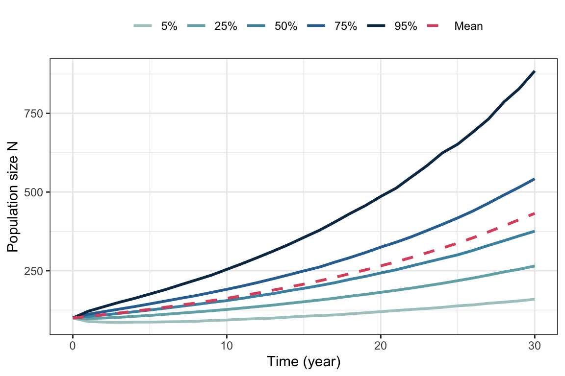
Figure 5.3: Percentiles and mean from 10000 simulated trajectories of the Lewontin-Cohen model with normally distributed annual growth rates with mean \(\lambda=1.05\) and standard deviation \(\sigma=0.1\).
In contrast to the realizations, the percentiles do not fluctuate (the higher the number of realizations, the more smooth they will be). The 50\(\%\) percentile represents the median and is therefore a good representation of the ‘typical’ population in the stochastic environment. The mean population size (shown in red on figure 5.3) is not a good measure of the typical population, because only only one or a few realizations reaching very high values can have a large impact on this value. Thus, for stochastic growth models the long-term growth rate of the median population is a better fitness measure than the long-term growth rate of the mean population. In extreme cases when the variance of the annual growth rates is large, the expected population size can increase exponentially because a few realizations reach extremely high values, while the median population size is declining and each realization will eventually go extinct with probability 1. We will get back to this below.
<br
5.3.2 The stochastic growth rate
First, we consider the growth rate of the mean population size, although we already know this is not the best measure for the typical population. Because we assumed that the \(\Lambda_t\)’s are IID (see above), the expected population size after \(t\) time steps is given by
\[\begin{align} \text{E}[N_t]&=N_0\text{E}\left[\prod_{i=0}^{t-1} \Lambda_i\right] =N_0\prod_{i=0}^{t-1}\text{E}[\Lambda_i] =N_0\lambda^t. \tag{5.2} \end{align}\]
Thus, the expected population size grows at the rate \(\lambda\) (the mean of the annual growth rate), just like a population growing exponentially in a constant environment. Note that \(\lambda\) does not depend on the variance of the annual growth rates.
To derive the long-term growth of the ‘typical’ population (the socalled stochastic growth rate) we look at the Lewontin-Cohen process (equation (5.1)) on log scale:
\[\begin{align} \ln N_t&=\ln \Lambda_{t-1}+\ln\Lambda_{t-2}+...+\ln\Lambda_{1}+\ln\Lambda_0+\ln N_0\\ &=\ln N_0+ \sum_{i=0}^{t-1} \ln \Lambda_i. \tag{5.3} \end{align}\] Here, the first term \(\ln N_0\) is a constant (since the initial population size is given). The second term is a sum over all the stochastic growth increments on log scale. Together with the IID assumption, this allows us to take advantage of the central limit theorem (if you need a reminder: https://en.wikipedia.org/wiki/Central_limit_theorem): As as the number of time steps \(t\) approaches infinity the sum will be normally distributed with mean \(t\text{E}[\ln\Lambda_t]\) and variance \(t\text{Var}(\ln\Lambda_t)\).
Thus, the expected value of \(\ln N_t\) is given by
\[\begin{align} \text{E}[\ln N_t]=\ln N_0 + \text{E}\left[\sum_{i=0}^{t-1} \ln \Lambda_i\right]=\ln N_0 + t\text{E}[\ln\Lambda_t] \end{align}\] This expectation grows (or declines) linearly over time \(t\), and the slope of this line is the mean \(\text{E}[\ln\Lambda_t]=r_s\). The constant \(r_s\) is called the stochastic growth rate (note that the name can be misleading, as this is a constant, and not a stochastic variable).
Importantly, the stochastic growth rate is generally lower than the growth rate of the mean population, \(r=\ln \lambda=\ln(\text{E}[\Lambda_t])\), unless the variance of the annual growth rates is zero (then they are the same). The stochastic growth rate describes the growth of the median population size. The population size \(N_t\) is lognormally distributed because \(\ln N_t\) is lognormally distributed (due to the central limit theorem), and the lognormal distribution is skewed. In the lognormal distribution median is always lower than (or equal to) the mean, and is a better descriptor of the central tendency (or as we put it, it provides a better description of a typical population growth trajectory than the mean).
How different are the two growth rates, and can we express this difference as a function of the variance of the \(\Lambda_t\), \(\sigma^2\)? Yes, Lewontin and Cohen (1969) showed (using a Taylor expansion of \(\ln \Lambda_t\) around \(\lambda\); not within the scope of this compendium) that the stochastic growth rate \(r_S\) can be written as
\[\begin{align} r_s\approx r-\frac{\sigma^2}{2\lambda^2}. \tag{5.4} \end{align}\] This equation tells us that the difference between the growth rate \(r\) in the constant environment and \(r_s\) in the stochastic environment is increasing with the value of \(\sigma^2\). Thus, we can have situations where the population growth rate \(r\) is positive, but \(r_S\) is negative. And in that case, extinction of the population (at some point) is certain.
5.3.3 Arithmetic and geometric mean
The stochastic growth rate \(r_s=\text{E}[\ln \Lambda_t]\) and the growth rate of the mean environment \(r=\ln \text{E}[\Lambda_t])\) can also be compared by considering the arithmetic and geometric mean of a series of annual growth rates \(\Lambda_t\). The arithmetic mean is given by
\[\begin{align} \lambda=\text{E}[\Lambda_t]=\frac{1}{t}\sum_{i=1}^t\Lambda_i, \end{align}\] and the log of this value is \(r=\ln \lambda\). The geometric mean is given by
\[\begin{align} e^{\text{E}[\ln\Lambda_t]}=\left(\prod_{i=1}^t \Lambda_i \right)^{1/t}, \end{align}\] and the log of this value corresponds to \(r_S=\text{E}[\ln\Lambda_t]\). In contrast to the arithmetic mean, the geometric mean depends on the variance \(\sigma^2\). The arithmetic mean will always be greater than or equal to the geometric mean, and in this case they are only equal in the constant environment (if \(\sigma^2=0\)).
The code below returns the arithmetic and geometric mean of a sequence of annual growth rates, and plots them along with the sequence:
AGMeans <- function(Tmax=100, mean.lambda=1.05, sd.lambda=.3){
  #Use lognormal distribution to avoid negative values
  Lambdavec <- rlnorm(n=Tmax,
                      log(mean.lambda)-
                        .5*log(1+ sd.lambda^2/
                                 (mean.lambda^2)),
                      sdlog=sqrt(log(1+sd.lambda^2/
                                       (mean.lambda^2))))
   geomLambda <- exp(mean(log(Lambdavec)))
   meanLambda <- mean(Lambdavec)
  data.frame("Time"=0:(length(Lambdavec)-1),
             "Lambda"=Lambdavec,
             "Geometric"=geomLambda,
             "Arithmetic"=meanLambda)
}
set.seed(20)

GetMeans <- AGMeans()
Geometric <- GetMeans$Geometric[1]
Arithmetic <- GetMeans$Arithmetic[1]
ggplot(GetMeans) +
  geom_point(aes(x=Time, y=Lambda), size=2, col=8)+
  geom_hline(yintercept= Geometric,lwd=1.2,
             linetype=2,col=2)+
  geom_text(aes(10, Geometric,
                label = "Geometric mean",
                vjust=2), col=2)+
  geom_hline(yintercept=Arithmetic,lwd=1.2,
             col=4)+
  geom_text(aes(10,  Arithmetic,
                label = "Arithmetic mean",
                vjust=-2),col=4)+
  theme_bw() +
  theme(legend.position = "none" )+
labs( x="Time (year)", y=expression(Lambda[t])) 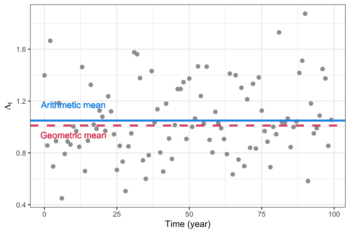
Figure 5.4: Arithmetic and geometric mean of a sequence of annual growth rates \(\Lambda_t\), with annual mean \(\lambda=1.05\) and annual standard deviation \(\sigma=0.3\)
5.3.4 Bet-hedging
From an evolutionary perspective, the Lewontin-Cohen model is an important starting point to describe fitness in a stochastic environment (\(r_S\)), and understand how it differs from the fitness in a the mean environment (\(r\)). In particular, it provides a baseline model to describe strategies of bet-hedging. Since \(r_S\) depends on both \(r\) and \(\sigma^2\), organisms in stochastic environments can improve their fitness through increasing the mean \(r\), or reducing the variance \(\sigma^2\). Bet-hedging strategies reduce the variance, at the cost of also reducing the arithmetic mean fitness. As a result the fitness in the stochastic environment \(r_S\) is optimized.
The study of bet-hedging started with the work of Cohen (1966) to understand the fitness of plants in unpredictable environments like a desert. Bet-hedging can operate through two main mechanisms, or a combination (Starrfelt and Kokko 2012):
Conservative bet hedging refers to strategies that ‘play it safe’, where the organism does not optimize its fitness for any given environment, but in the long run still come out with a higher geometric mean fitness. For instance, a bird could lay a low number of eggs at each reproduction to improve the survival of their offspring, thus reducing the variance but at the cost of a lower than optimum clutch size in the mean environment.
Diversifying bet-hedging are strategies that avoid risk by ‘not putting all eggs in one basket’, for instance by producing offspring with a high diversity of phenotypes. While this will certainly increase the variance in fitness among the offspring, it reduces the variance of the parent. Again, it is not truly bet-hedging unless the parent also pays a cost in terms of lowered arithmetic mean fitness (here corresponding to producing offspring of just one type optimal for the mean environment).
5.4 Stochastic growth of structured populations
In structured populations, the stochastic population dynamics are more complex because the annual population growth rates are no longer ‘IID’ (Independently and Identically Distributed). For the Lewontin-Cohen model this was a key assumption that allowed us to use the central limit theorem to derive the stochastic growth rate. But in structured populations, the annual growth rates will show autocorrelation (a memory in the process) because the population structure itself generates lags in the growth process. Even if there is some stochastic environmental variable that is IID and gives rise to stochasticity in the population growth, the population growth rates will not be IID.
For instance, if the environment is particularly good for reproduction one year, this can lead to a ‘strong’ year class (cohort) that persists in the population over time and affects the population growth rate for potentially many years. We get ‘waves’ of such cohorts that generate long-term fluctuations in the stage structure on top of the year-to-year fluctuations due to stochasticity. The long-term fluctuations create autocorrelation in the population growth process. In contrast to the population growth in a constant environment, where the transient initial fluctuations disappear over time (chapter 3), the transients will never really disappear in a stochastic environment Instead, the population structure will fluctuate around the stable structure.
How can we then study population growth and fitness of structured populations in stochastic environments? We can always do simulations (projections) of the population growth process, as we did for the Lewontin-Cohen model, and we can define the stochastic growth rate based on a (long) sequence of generated populaton sizes. In addition, under the assumption of small fluctuations it is possible to approximate the stochastic growth rate as a function of the mean, variance and covariance of matrix elements, as we will see below. First we will define a general model to describe the growth of structured populations in a time-varying environment.
5.4.1 Defining the process
In a fluctuating environment, the projection matrix \(\mathbf{A}\) will take a new value each time step, so that the population growth over many time steps is given by matrix multiplication from time 0:
\[\mathbf{n}_{t+1}=\mathbf{A}_{t}\mathbf{n}_{t}=\mathbf{A}_{t}\mathbf{A}_{t-1}\mathbf{A}_{t-2}\cdots\mathbf{A}_{0}\mathbf{n}_{t}\]
When these time-dependent projection matrices \(\mathbf{A}_t\) are generated by a random process each time step, we have a stochastic matrix model. There are two main approaches to study the dynamics of such a model:
The environment-blind approach generates a set of projection matrices e.g. from each year of a study, and then samples among these to generate a new stochastic sequence of matrices according to a given sampling model (e.g. a Markov process). In this case, correlation between vital rates of the projection matrix are automatically incorporated since the entire matrix is sampled.
The environment-specific approach specifies each matrix element (e.g. fertility and survival coefficients) as a stochastic variable with a mean, variance and potentially covariance among matrix elements. Together, all the stochastic elements in the model define a multivariate vector with a given distribution (specified by a vector of means and a variance-covariance matrix). This approach is more complex, but often better suited to account for explicit relationships between the vital rates and environmental variables such as temperature.
Bird example
We will again use the bird example introduced in @ref{birdtable} and following chapters, and now consider a stochastic version of the matrix model for this bird with pre-reproductive census (chapter 3).
In the constant environment, the pre-reproductive projection matrix for the songbird was given by ((3.6)):
\[\begin{align} \begin{split} \mathbf{A}=\left[\begin{matrix} f_1 & f_2 &f_3 \\ s_1 &0&0\\ 0 & s_2 &0 \\ \end{matrix}\right]=\left[\begin{matrix} 0 &0.6 &1.2 \\ 0.9 &0&0\\ 0 & 0.6 &0 \\ \end{matrix}\right]. \end{split} \end{align}\]
We will now add stochasticity to the elements of this matrix, by allowing the fertilities and survival probabilities to fluctuate randomly. Adding stochasticity needs to be done with some care: Survival probabilities are restricted to be between 0 and 1, and fertilities must always be non-negative. A good idea is to use appropriate scaling functions (link functions) where stochasticity can be added as a normally distributed variable on the link scale. For this example, we will assume a log-link function for the fertilities, and a log log link function for the survival (but in general many other kinds of functions are also possible):
\[f_{it}=\exp(\beta_{fi}+\varepsilon_{fit})\]
\[s_{it}=\exp(-\exp(-\beta_{si}-\varepsilon_{sit}))).\]
Here \(\varepsilon_{fi}\) and \(\varepsilon_{si}\) are random (stochastic) variables assumed to follow a normal distribution with mean 0 and standard deviation \(\sigma_{fi}\) and \(\sigma_{si}\), respectively. The constants \(\beta_{fi}\) and \(\beta_{si}\) define the fertility and survival when the standard deviations (and thus the \(\varepsilon\)’s) are zero. Note that this is just one of several ways to model stochasticity in survival and fertility.
Plot one realization of the process
To add stochasticity to the fertilities and survival probabilities in the projection matrix, we will use the function mvrnorm() from the package MASS, which generates values from the multivariate normal distribution. The function mvrnorm uses a variance-covariance matrix as one of its input variables, and here we will for simplicity assume no covariance. We also assume that stochasticity only affects survival and fertility coefficients, and that these follow log-log link and log-link functions, respectively.
The following function generates a series of random projection matrices using the mvrnorm() function from the package MASS to add stochasticity in survival and fecundity. The matrices are returned as an array, which is an extension of the ´matrix´ object to multiple dimensions. Here we have three dimensions: Time (Tmax), \(k\) and \(k\), where \(k\) is the number of rows and columns of the projection matrix.
Inputs to the function are the projection matrix in the constant environment \(\mathbf{A}\), its main components \(\mathbf{U}\) and \(\mathbf{F}\) (used to separate out survival coefficients and fertilities), and two vectors defining the variance in scaled fertility and survival. Each vector needs to be of length \(k\) corresponding to the number of stages in the population.
Amat.array <- function(MatA,
                       MatU,
                       MatF,
                       tmax=30,
                       VarF=rep(0.03, 3),
                       VarS=rep(0.03, 3)){
  #Split survival/transition matrix:
  SplitU <- DecomposeU(MatU)
  #Split fertility matrix:
  SplitF <- DecomposeF(MatF)
   #Transition matrix:
  Gmat <- SplitU$Gmat
   #Survival vector:
  Svec <- SplitU$Survival
  #Define beta (log-log link function):
  Beta.S <- -log(-log(Svec))
  #Offspring transition matrix:
  Qmat <- SplitF$Qmat
  #Fertility vector:
  Fvec <- SplitF$Fertility
  #Define beta (log link function):
  Beta.F <- log(Fvec)

  #variance covariance matrix
  SigMat <- diag(c(VarS, VarF))
  #Draw random (scaled) values for S and F:
  SFTime <- mvrnorm(tmax, mu=c(Beta.S, Beta.F), Sigma=SigMat)
  #Number of matrix classes
  k <- length(Svec)
  #Rescaled survival probabilities (loglog link):
  SvecTime<-   exp(-exp(-SFTime[,1:k]))
  #Rescaled fertilities  (log link):
  FvecTime<- exp(SFTime[,(k+1):(2*k)])
#Build  projection matrix for each time step:
  A.array <- array(NA,dim=c(k,k,tmax))
  for (i in 1:tmax){
    Smat <- diag(SvecTime[i,])
    Fmat <- diag(FvecTime[i,])
    A.array[,,i] <-   Gmat%*%Smat+Qmat%*%Fmat
  }
return("Amats" = A.array)
}
Using this function to generate a sequence of stochastic projection matrices, we can make another function to project the population growth over time. This projection is similar to the one we used for the constant environment (chapter 3), except that for each time step we now use a new different matrix due to stochasticity. The function below returns a data frame with the size of each stage over time, including the initial sizes provided in n0.
projection.stochastic <-function(Amats, n0){
    Tmax <- dim(Amats)[3]
    k <- dim(Amats)[1]
    if(length(n0)!=k){
      warning("n0 should have length k
              corresponding to number of
              stages in the Amats object")
      }
    Nmat <- matrix(NA,nrow= Tmax+1, ncol=k)
    Nmat[1,] <- n0
  cnames <- paste("n", 1:k, sep="")
  timesteps <- 0:Tmax
    for(i in 2:(Tmax+1)){
        Nmat[i,] <- Amats[,,i-1] %*% Nmat[i-1,]
        }
  frame <- data.frame(timesteps,Nmat)
  colnames(frame) <- c("time", cnames)
  frame
}
Bird example
set.seed(20)

#Generate sequence of stochastic matrices:
Amats.bird <- Amat.array(MatA=Abird.pre,
                         MatU=Ubird.pre,
                         MatF=Fbird.pre,
                         tmax=20,
                         VarF=rep(0.03, 3),
                         VarS=rep(0.03, 3))

#Project growth:
stochastic.bird <- projection.stochastic(Amats = Amats.bird,
                                         n0=rep(10,3))

#Long format for plotting:
stochastic.bird.long <- stochastic.bird %>% pivot_longer(c(-time),
               names_to = "AgeClass", values_to = "Value")

#Plot:
ggplot(stochastic.bird.long) +
  geom_line(aes(x=time, y=Value, col=AgeClass,
                linetype=AgeClass), lwd=1.2)+
  geom_point(aes(x=time, y=Value, col=AgeClass), size=3)+
  theme_bw() +
  scale_color_manual(values=colors3)+
  scale_linetype_manual(values=c(1,2,3))+
  labs( x="Time (year)", y="Age class size")+
  theme(legend.position = "top" )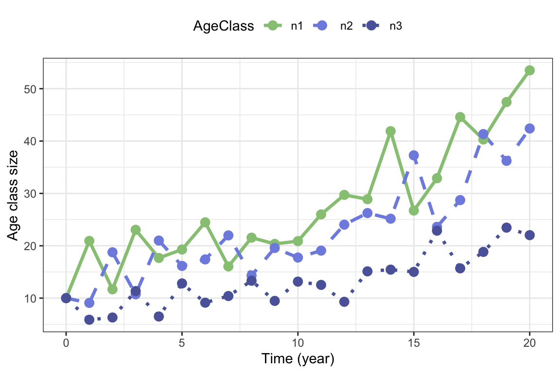
Figure 5.5: One realization of stochastic growth in the bird example with pre-reproductive census, with stochastic survival and fertility coefficients.
Figure (fig:birdstochastic1) shows the growth of each stage of the bird population over 20 years, starting from a population with 10 birds in each age class.The highest number of fluctuations is found for the first age class, and we can see that the peaks in this age class are followed by peaks in year class 2 and 3 in the following years, as the cohort grows through the population.
We can also plot the total population size, by summing up the values of the age classes for each year, as shown in figure 5.6:
#Sum up population sizes
stochastic.bird$Ntot <- apply(stochastic.bird[,-1],1,sum)

ggplot(stochastic.bird) +
  geom_line(aes(x=time, y=Ntot), lwd=1.2)+
  geom_point(aes(x=time, y=Ntot), size=3)+
  theme_bw() +
labs( x="Time (year)", y="Populatipn size N") 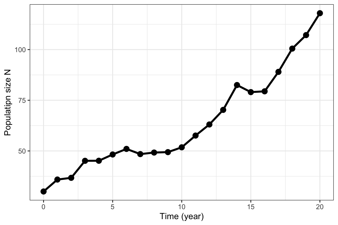
Figure 5.6: Same process as in figure 5.5, with age classes summed up to get the total population size.
Plot many realizations of the process
Instead of looking at just one realization of the stochastic growth process, it is often useful to generate multiple realizations and look at summary statistics and properties for these, as we have seen already for the Lewontin-Cohen-process.
The following function generates a series of matrices nsim times, each series of length Tmax, and returns the projected total population size over time for each series, in a data frame. Other input variables are the constant matrices and variance vectors, and initial population vector.
nsim.stochastic <- function(nsim=100,
                            tmax=30,
                            n0=rep(10,3),
                            MatA,
                            MatU,
                            MatF,
                            VarF,
                            VarS){
  frame <-  data.frame("Time"=0:tmax)
  for(m in 1:nsim){
  AMATS <- Amat.array(MatA=MatA,
                      MatU=MatU,
                      MatF=MatF,
                      VarF=VarF,
                      VarS=VarS,
                      tmax=tmax)
   projectN <- apply(projection.stochastic(Amats=AMATS,
                                           n0=n0)[,-1],1,sum)
  frame <- cbind(frame, projectN)
  names(frame)[m+1] <- paste("Rep",m,sep="")
  }
  frame
}
Bird example
We can now plot multiple realizations also in the bird example, as shown in figure 5.7
set.seed(20)

nsim.bird <- nsim.stochastic(MatA=Abird.pre,
                             MatU=Ubird.pre,
                             MatF=Fbird.pre,
                             VarF=rep(0.03, 3),
                             VarS=rep(0.03, 3),
                             tmax=20, nsim=100,
                             n0=rep(10,3))


nsim.bird.long <- nsim.bird %>% pivot_longer(c(-Time),
               names_to = "Rep", values_to = "N")

ggplot(nsim.bird.long) +
  geom_line(aes(x=Time, y=N, col=Rep), lwd=.5)+
  scale_color_manual(values=rep(1,100))+
  theme_bw() +
   theme(legend.position = "none" )+
labs( x="Time (year)", y="Population size N") 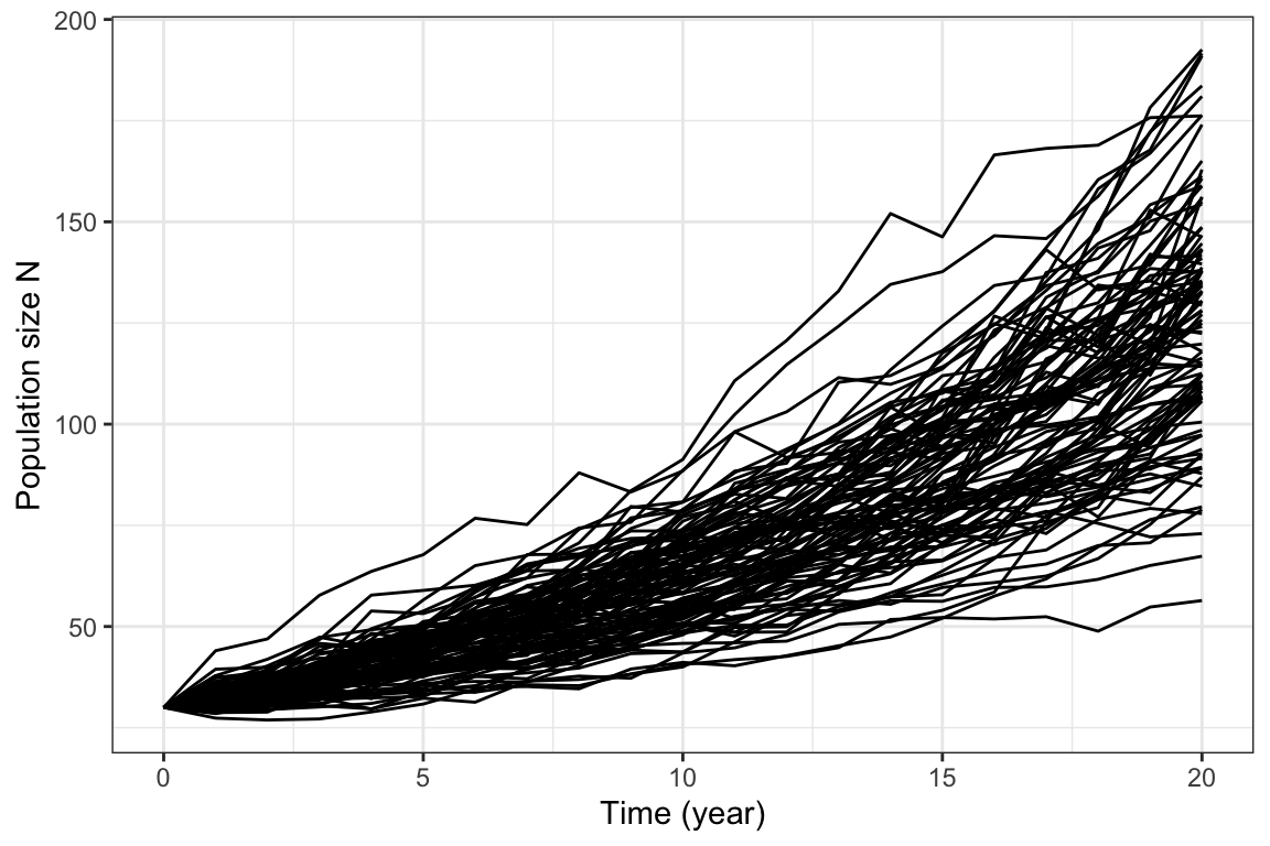
Figure 5.7: 100 realizations of the stochastic bird growth process with same parameters as in figure 5.6.
To estimate the stochastic growth rate \(r_S\) from multiple realisations, we can use the following function (this measure is based on the mean of the annual growth increments of \(\ln N\)):
diffmat <- apply(log(nsim.bird[,-1]),2,diff)
rS <- mean(apply(diffmat,2,mean))
In this example, the stochastic growth rate is \(r_S\approx\) 0.07.
Plot percentiles from many realizations
As shown for the Lewontin-Cohen model we can also plot percentiles of the stochastic population trajectories from a structured model, after running multiple realizations.
Bird example
For the bird example with 20 time steps, we get
set.seed(20)

#Apply function to get 10 0000 realizations (can take some time)
simbird_Large <- nsim.stochastic(MatA=Abird.pre,
                                 MatU=Ubird.pre,
                                 MatF=Fbird.pre,
                                 VarF=rep(0.03, 3),
                                 VarS=rep(0.03, 3),
                                 tmax=20,
                                 nsim=10000,
                                 n0=rep(10,3))

#Get the 5, 25, 50, 75, and 95 percentiles:
Percentiles2  <- t(apply(t(simbird_Large[,-1]),
                         2,
                         quantile,
                         probs=c(.05, .25, .5, .75,.95)))


#Store percentiles in data frame
BirdPercentiles <- as.data.frame(cbind("Time"=0:(dim(Percentiles2)[1]-1),
                                       Percentiles2))

BirdPercentiles$Mean <- apply(t(simbird_Large[,-1]),2, mean)

#Make long format for plotting
BirdPercentiles.long <- BirdPercentiles %>% pivot_longer(c(-Time),
               names_to = "Percentile", values_to = "N")

#Make sure the order of the percentiles is correct
BirdPercentiles.long$Percentile <- factor(BirdPercentiles.long$Percentile,
                    levels=c("5%", "25%", "50%", "75%", "95%","Mean"))

ggplot(BirdPercentiles.long) +
  geom_line(aes(x=Time, y=N, col=Percentile,
                linetype=Percentile), lwd=1)+
  scale_color_manual(values=c(colors5,2))+
   scale_linetype_manual(values=c(rep(1,5),2))+
  theme_bw() +
   theme(legend.position = "top",
         legend.title = element_blank())+
  labs( x="Time (year)", y="Population size N") +
   guides(color = guide_legend(nrow = 1, byrow = TRUE))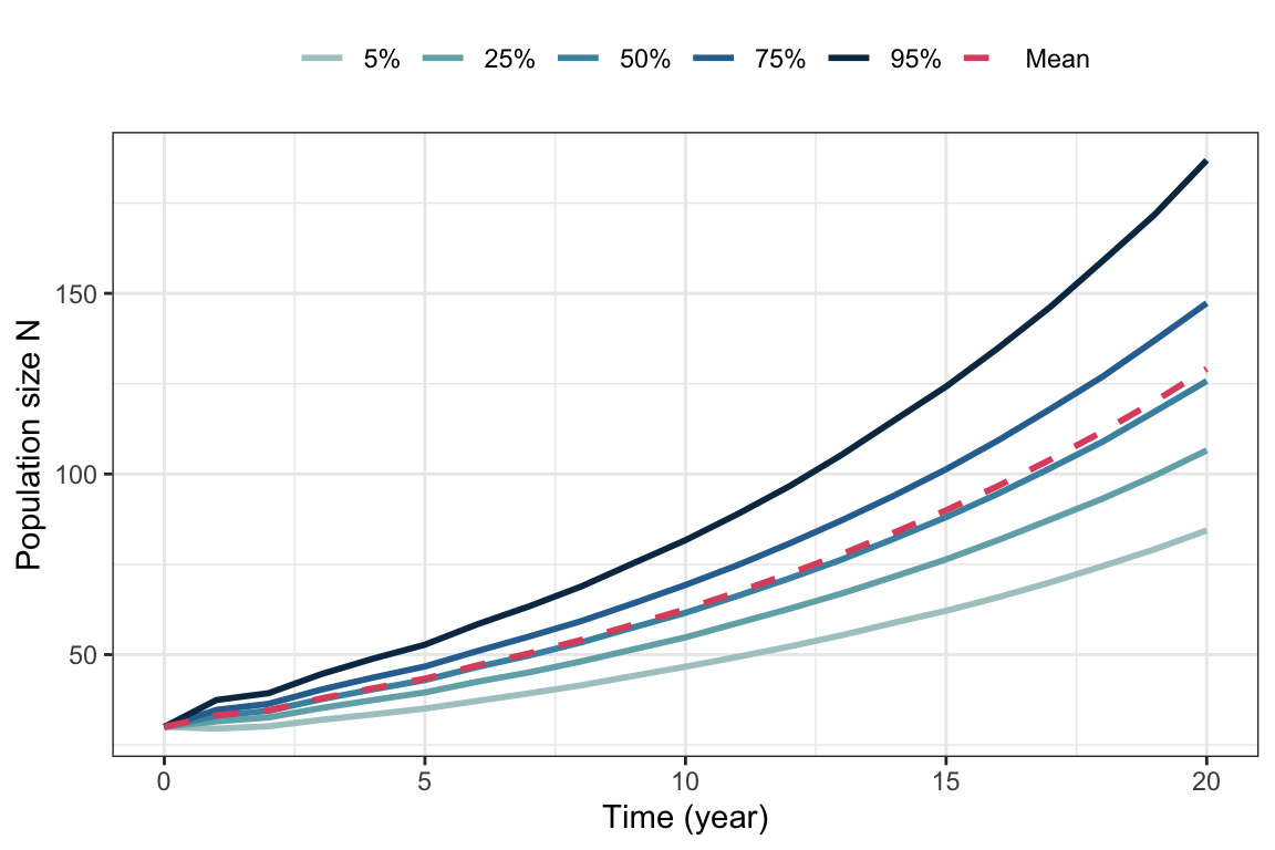
Figure 5.8: Percentiles and mean from 10000 simulated trajectories of the stochastic bird model, with same parameter values as in figure 5.6.
5.4.2 Stochastic growth rate
When a stochastic sequence of projection matrices is available, it can be used to project the population size over time, and the stochastic growth rate can be defined from the resulting population process as the asymptotic time-averaged growth rate:
\[\begin{align} r_S=\lim_{t\to\infty}\frac{1}{t}[\ln N_t-\ln N_0], \tag{5.5} \end{align}\] This value can easily estimated from simulations, once the sequence of stochastic matrices is determined.
The following code can be used to calculate the stochastic growth rate following the definition of equation (5.5), given a sequence of projection matrices. The cutoff argument removes the first time steps (corresponding to cutoff number), where transient fluctuations can be large unless the population starts at the stable distribution.
EstimateSGR <- function(Amats, n0, cutoff=20){
  Tmax <- dim(Amats)[3]
    if(cutoff>=Tmax){
      warning("cutoff must be lower
              than the number of
              matrices in Amats")
      }
  project <- projection.stochastic(Amats=Amats, n0=n0)
  Ntot <- apply(project[,-1],1,sum)
  logN <- log(Ntot[cutoff:length(Ntot)])
  TM <- length(logN)
  (logN[TM]-logN[1])/TM
}
Note that the estimate becomes more accurate the longer the sequence, and the closer the initial population vector is to the stable distribution from the constant (mean) environment (or the higher the cutoff). If the growth rate is very large or small, numerical issues can arise affecting the estimation.
This estimate is based on only one run of the process, and the accuracy can be improved by running it many times.
Bird example
Applying the function in the bird example (for a longer sequence of 1000 projection matrices), we get the following estimate of the stochastic growth rate:
set.seed(25)
#Generate sequence of stochastic matrices:
Amats.bird2 <- Amat.array(MatA=Abird.pre,
                          MatU=Ubird.pre,
                          MatF=Fbird.pre,
                          tmax=1000,
                          VarF=rep(0.03, 3),
                          VarS=rep(0.03, 3))

#Estimate growth rate
rs.bird <- EstimateSGR(Amats = Amats.bird2,
                       n0=rep(10,3))

round(rs.bird, 4)
## [1] 0.0704This means that \(r_s\approx\) 0.0704 for the bird example. In the constant environment we had \(r= \ln\lambda\approx\) 0.068 (you can check that you get approximately this value by setting the variances to zero in the above function).
5.4.3 Small noise approximation
So far we have relied on simulations of the population process to estimate the stochastic growth rate, which does not provide a good understanding of how it depends on the variance and covariance of the underlying matrix elements.
Assuming small environmental fluctuations (i.e. that no projection matrix would be very different from the mean matrix), Tuljapurkar (1982) derived the following useful approximation for the stochastic growth rate that links it to the underlying matrix elements:
\[\begin{align} r_S&\approx r-\frac{1}{2\lambda^2}\sum_{i}\sum_{j}\sum_{k}\sum_{l}\frac{\partial\lambda}{\partial a_{ij}}\frac{\partial\lambda}{\partial a_{kl}}\text{Cov}(A_{ij},A_{kl})\\ &= r-\frac{1}{2\lambda^2}\sigma_e^2. \tag{5.6} \end{align}\]
We see that equation (5.6) is similar to the approximation of the Lewontin-Cohen model (equation (5.4)), which is not strange since they are both based on a Taylor approximation (mathemtacal details are outside the scope of this compendium). THe small noise approximation is useful because it shows how the stochastic growth rate is related to the sensitivities of the mean projection matrix, and the variances (and covariances) between matrix elements.
The small noise approximation is relevant to the topic of demographic buffering. Demographic buffering, or simply ‘buffering’, refers to the common observation that vital rates to which \(\lambda\) (in the mean environment) shows a high sensitivity in the mean environment often show low temporal variability. This is often seen as a strategy to mitigate negative impacts of variability, which would be most severe if it affected these vital rates that are so important to the growth in the average environment. However, because the variance of vital rates is mathematically constrained by the mean (e.g. for survival, a high mean automatically implies that the variance must be low) it is difficult to tease appart the underlying mechanisms behind an observed low variance and high mean for any given vital rate. In contrast to bet-hedging, buffering refers to any case of low variation in vital rates, without any assumption about any cost to the mean.
5.5 Exercises
Exercise 5.1
Start with the flowering plant from exercise 2.2 and exercise 3.2. Assume a pre-reproductive census, and use the following projection matrix for the mean environment (increased fecundity to get \(\lambda>1\)):
x <- 0:4
nx <- c(12376, 4233, 1790, 340, 268)
mx <- c(0, 0, 0, 2.1, 3.2)
lx <- nx/nx[1]
px <- c(lx[2:5]/lx[1:4],0)

C <- 8

APlant <- Create.Amat(Svec=px[2:5] , Fvec=px[1]*mx[2:5]*C)
FPlant<- UPlant<- APlant

FPlant[-1,] <- 0
UPlant[1,] <- 0

round(APlant,3)
## [,1] [,2] [,3] [,4]
## [1,] 0.000 0.00 5.746 8.756
## [2,] 0.423 0.00 0.000 0.000
## [3,] 0.000 0.19 0.000 0.000
## [4,] 0.000 0.00 0.788 0.000Add stochasticity to the fertility coefficients using the same approach as for the bird example in this chapter, and make some plots of the projected growth of the age classes for different values of the variances. Interpret what happens.
Add stochasticity to the survival coefficients instead (but not in fertility) and make some plots of the projected growth as in the previous point. Do you notice a difference?
Think about possible bet hedging strategies the plant could use to optimize fitness in a varying environment. Do you see any signs of bet-hedging in its current life history?
Exercise 5.2
Consider the black-headed gull example from chapter 4.4.2, with two different habitats. Instead of the migration pattern described in the example (where offspring migrate), assume that migration is random between the two environments, so that each year each gull ends up in either habitat by chance. The two projection matrices describing each habitat are given by
\[\begin{align*} \mathbf{A}_{\text{good}} &=\left[\begin{matrix} 0&0.096& 0.16&0.224&0.32\\ 0.8&0& 0& 0&0\\ 0&0.82& 0& 0&0\\ 0&0& 0.82& 0&0\\ 0&0& 0& 0.82&0.82 \end{matrix}\right], \end{align*}\]
and
\[\begin{align*} \mathbf{A}_{\text{poor}} &=\left[\begin{matrix} 0&0.1& 0.16&0.2&0.2\\ 0.8&0& 0& 0&0\\ 0&0.82& 0& 0&0\\ 0&0& 0.82& 0&0\\ 0&0& 0& 0.82&0.82 \end{matrix}\right]. \end{align*}\]
What is the value of \(\lambda\) in each habitat?
Write an R function that returns a series of gull projection matrices for a given number of time steps (returned as an array where the third dimension is time), assuming a random draw each year (hint: the function
sample()can be used to make random draws. For instance,sample(c("A", "B"), 10, replace=TRUE)will return a vector of 10 values of either “A” or “B”.).Calculate the mean growth rate and the stochastic growth rate for the black-headed gull assuming such random migration between the habitats. Make a quantile plot of population growth and highlight the growth trajectories corresponding to growth of the median and mean population.
In the
sample()function there is an argumentprobthat can be used to set different probabilities for each environment. For instance, withsample(c("A", "B"), 100, replace=TRUE,prob=c(.8, .2))there is a probability of 0.8 of drawing an “A” and 0.2 of drawing a “B” for each sampling event, resulting in many more “A”’s over time. Modify the previous code and consider what happens to the population growth if the probability of ending up in the good environment is higher, or lower.